For some time I have been looking for a good model or basis for estimating path loss of radio signals over water. This article presents four possible models that could be useful in predicting path loss over water at VHF frequencies.
I found some data about VHF radio propagation over water in the Federal Communication Commission (FCC) regulations for PART 80--STATIONS IN THE MARITIME SERVICE. The commission has provided some charts for the purpose of calculating the coverage of a shore station. A chart showing anticipated signal levels with over distance for various antenna heights allows deduction of path loss; the chart appears in Part 80.767 and is labeled "Propagation Curve."
The chart is very interesting because it shows signal loss with distance with several curves. There is a plotted line labeled "Free Space", which represents the theoretical best-case loss curve for a radio wave traveling a certain distance. There are also curves for real-world situations, with various antenna heights.
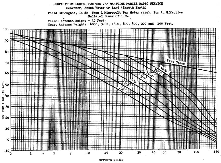
Figure 1. Graph of signal strenth versus distance for various antenna heights. From FCC Part 80 regulations.
The curves show that for very short distance paths and very tall antennas, the path loss in the real world is the same as in free space, but once the path distance becomes more than a few miles, the characteristics of the path loss change remarkably.
I investigated this chart to see if I could deduce the path loss factor for the distance that was being used. I will describe my method. First, I looked closely at the free-space curve. I found the signal levels (dBu) for the distances (d) of 10 and 100 miles.
Miles  dBu
 10    83
 100   63
When the distance changed by a factor of ten, the signal decreased by -20dB. This suggests the relationship is
 dB = x log(d)
-20 = x log(10)
  x = -20 / log(10) = -20
This is exactly what would be expected. The factor -20 log(d) is used in the free-space model of path loss.
Next, I investigated the other curves to see what sort of relationship between signal level and distance they represented. (Note that the x-axis in the chart is using a logarithmic scale.) Using the curve for an antenna of 100-feet, I used distance values of 5 and 50, where the slope of the curve appeared to be constant. I found the following values of signal and distance:
Miles  dBu
  5    75
 50    19
When the distance increased by a factor of ten the signal decreased by -56 dB. This suggests the relationship of path loss and distance must be:
 dB = x log(d)
-56 = x log(10)
  x = -56 / 1 = -56
The curve on the chart seems to show that when when the distance between stations exceeds a few miles the path loss as a function of distance behaves according to the relationship dB = -56 log(d). This model describes a relationship between signal and distance where the path loss increases at a rate that is significantly more lossy than in free space. In another article, Estimating Path Loss on Marine Non-Line-of-Sight Paths, the path loss factor was found to be often cited in the range of -40 log(d) to perhaps -46 log(d), which is less than the -56 log(d) suggested by the FCC propagation chart.
We can also see the effect of antenna height on signal strength by using the chart data at a particular distance, and noting the change in signal strength with antenna height. For example, examine the several curves of signal strength on the chart at a distance of 10-miles. The signal strength varies in proportion to antenna height as follows:
Antenna Height  Signal strength
100-feet        60-dBu
200-feet        66-dBu
400-feet        73-dBu
We see that when the antenna height is doubled, the signal strength increases by 6-dB, a factor of four, or more. This is a surprising result. We will see this repeated in the next model, Egli's Model, presented below.
The FCC's chart is part of a procedure to establish the coverage area of shore stations, so the intent may be to use a method that will result in a coverage area that is very reliable. This may explain why the propagation loss for distance is predicted to be much greater than the free space model would suggest.
In my earlier article (hyperlinked above) I estimated the path loss based on my estimate of the signal level received for a particular station, WXN69. I estimated the signal level received was -97 dBm. This was just a rough estimate, based on the receiver having a rated sensitivity for a 10dB SINAD at a signal of -107 dBm, and judging (by ear and experience) the received signal to be perhaps 10dB stronger than that minimum signal level. If the signal level I observed were actually at the -107 dBm level, then the path loss equation derived from that estimate would have needed a distance factor of -51.6 log(d) for (d) in miles. That value is not too far off from the FCC chart curve's behavior, which seems to suggest -56 log(d) is the appropriate model.
The FCC Part 80 chart makes clear that the free-space model estimate is not appropriate unless the path is very short and has a lot of ground clearance (to eliminate the influence of the ground and any reflections). It is also clear that any estimate of the effect of distance on path loss that suggests it will less the -40 log(d) is much too optimistic and probably completely unrealistic.
I am sure that at this point some readers—if there are any readers at all—are probably wondering what I am talking about. Let me explain a bit more in detail. When the signal loss or path loss for a certain distance is described as being
20 log(d)
we are saying that the path loss increases with distance according to that rate. Let us explore the increase in path loss when the path length doubles, as in a path of 10-miles increasing to a path of 20-miles. The path loss due to distance will be:
For 10-miles

loss = 20 log(10)
loss = 20 dB

For 20-miles

loss = 20 log(20)
loss = 26 dB
When the path distance doubled, the path loss changed 6 dB. Because there was decrease in signal, we say the path loss changed -6 dB. The notation -6 dB represent a ratio. In terms of a ratio of power, we can find the power ratio from the definition of dB for power, which is
dB = 10 log (P1/P2) where P1, P2 are two power levels
We can also evaluate that relationship to find the power ratio represented by the dB expression. That becomes
(P1/P2) = 10^(dB/10)
Now we evaluate for -6 dB to find the ratio of powers:
(P1/P2) = 10^(-6/10)
(P1/P2) = 10^-0.6
(P1/P2) = 0.25
In other words, when the path distance doubled, the signal power decreased to 0.25 of the original power, or one-fourth the original power. This is another way of describing the inverse square law relationship. I think many readers will be familiar with that behavior, but may have not realized that it was represented in the notation 20 log(d).
When models for propagation use a factor for distance of 20 log(d), they are assuming that the decrease in signals will just obey a simple inverse square law relationship. This is the behavior that would occur in free space, an ideal environment in which nothing else affects the radio wave as it propagates. In the real world there are other factors in the environment that affect the signal loss in propagation, causing the real-world signal decrease to be greater. This behavior is reflected in having a path loss model in which the distance factor is greater than 20log(d).
More investigating into path loss models permitted me to come across a reference to the c.1957 work of Egli, who proposed that path loss could be calculated by the relationship of:
Pr = 0.66*Gb*Gm * [(Hb*Hm)^2/d^4] *[40/f]^2 *Pt

where

Pr = received power
Pt = transmit power
Gm = gain of mobile antenna (not in dB)
Gb = gain of base antenna (not in dB)
Hm = height of mobile antenna (meters)
Hb = height of base antenna (meters)
d = path distance (meters)
f = Mhz
This model contains several significant observations:
For more on Egli's model, and propagation path loss models in general, see Radio Propagation Models, an outline of a course in Electrical Engineering from Harvard Univerity.
Egli's model is not very optimistic about a typical boat-to-boat path. Using the following input:
Antenna gain = 2 for both antennas, i.e. 3-dB
Antenna height = 3-meters, i.e. about 10-feet, for both antennas
Transmitter power = 25-watts
Frequency = 156-MHz
the model calculates the received signal power as follow
Miles   dBm
0.6 = -92.7
1.2 = -104.8
2.5 = -116.8
4.9 = -128.9
As you can see, when the distance doubles the path loss increases by 12dB, which is what is suggested by the 40log(d) factor.
A really good receiver sensitivity is 0.25-microVolt, which is a signal level of -119 dBm. Egli's model suggests that we will reach that signal level at a range of only 2.5-miles. The model does much better when antenna height is increased. For example, if one antenna is raised to 10-meters (33-feet), then the path distance for a -116.8 dBm received signal doubles to about 5-miles.
The model is for propagation over smoothly rolling terrain with about 50-foot variation, so calm seawater will probably be provide a better path, that is, have lower path loss. The model is also statistical; it predicts a path loss that occurs about half the time.
I also found an on-line calculator that is said to use the Egli model. And I built my own spreadsheet version of an Egli's calculator. It shows very good agreement with the on-line calculator (linked above) if the 0.66 factor is removed. That factor was probably to account for statistical probabilities.
Using the on-line calculator based on Egli's model (linked above), the path loss for the following situation
Antenna Height-1 = 100-feet (e.g., a shore station)
Antenna Height-2 = 10-feet (e.g., a small boat)
Frequency = 157-MHz
Transmission distance = 30-miles
is calculated to be -160 dB. We can now predict the signal level we might have for this path if we have the following characteristics in each station:
Transmitter power = 25-Watts
Antenna gain = 3 dB
A transmitter power of 25-Watts is a signal of +44 dBm. Both the transmit antenna and the receive antenna have 3-dB gain. We can now predict the received signal level as follows:
TxPower + TxAntGain + RxAntGain = PathLoss = RxPower

+44dBm + 3dB + 3dB + -160dB = -110 dBm
A received signal level of -110 dBm in a 50-Ohm system corresponds to a 0.7-microVolt of signal. Most modern VHF Marine Band radios have receivers with sensitivity of 0.5-microVolt for 10-dB SINAD, so the received signal on this path should be above the receiver's rated sensitivity.
For the path loss, transmitter power, antenna gains, and receiver sensitivity described above, the Egli's model predicts a useable signal at a range of 30-miles. Egli's model is based on gently rolling terrain over land with hills not more than 50-feet high. On an all-water path with no intervening terrain, the Egli's model should be a reasonably accurate predictor of radio coverage, especially over saltwater and calm seas.
The ITU has a recommendation publication that covers radio propagation predictions, Recommendation ITU-R P.1546-5 (09/2013), Method for point-to-area predictions for terrestrial services in the frequency range 30 MHz to 3 000 MHz. This publication provides several graphs showing signal strength change with distance over a variety of paths. Of interest to this discussion is Figure 4, which shows signal change as a function of distance for path over seawater at 100-MHz. One station has an antenna height of 10-meters (33-feet), and the chart plots received signal strength for various antenna heights at the second station.
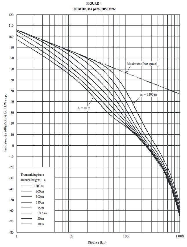
Figure 2. Graph of signal strenth versus distance for various antenna heights. From ITU-R P.1546-5.
Inspecting the chart for the change in signal strength with change in distance, we see the following apparent values for rate of change of signal as a function of distance:
At distance 2-km, signal is 87.5 dBu
At distance 20-km, signal decreases to 50 dBu
For change in distance of ratio 10, signal decrease is ratio -37.5 dB
Solving this for our expression in the form dB = x log(d) gives

dB = 37.5log(d)

At distance 20-km signal is 50 dBu
At distance 30-km signal is 41 dBu
For change in distance of ratio 1.5, signal decrease is ratio -9 dB
Solving this for our expression in the form dB = x log(d) gives

dB = 51(log)d
This change in rate of attenuation is reflected in the changing slope of the curves. For shorter paths, the rate of signal decrease is not as great as on longer paths.
We can also look at the effect of antenna height change. There are several curves where the antenna height is doubled between curves.
For the curve for h = 75m at distance 30-km, signal is 55 dBu
For the curve for h = 150m at 30-km, signal is 61 dBu
When antenna height was doubled, signal increased 6 dB
Based on these curves, we that a distance of 30-km, doubling the antenna height causes a very substantial 6 dB increase, or a four-fold gain in received signal power.
The National Telecommunications and Information Administration (NTIA), a government agency that I had never heard of, published an interesting technical report in August 1997 titled "Assessment of Compatibility Between 25 and 12.5 kHz Channelized Marine VHF Radios, NTIA TR 97-343." As part of their investigation, a model for path loss of VHF signal propagation over seawater was necessary. The report used "the NTIA nlambda propagation model for smooth earth at 157.1 MHz over seawater with vertical polarization at the 50 percentile." A formula for the model was not provided, but three graphs that showed path loss between two typical ship stations were provided; path loss was plotted for antennas at two differnent practical heights, 3-meters and 10-meters, as seen below. The 10-meter height is considered typical for a commercial vessel, and the lower 3-meter height is for recreational vessels.
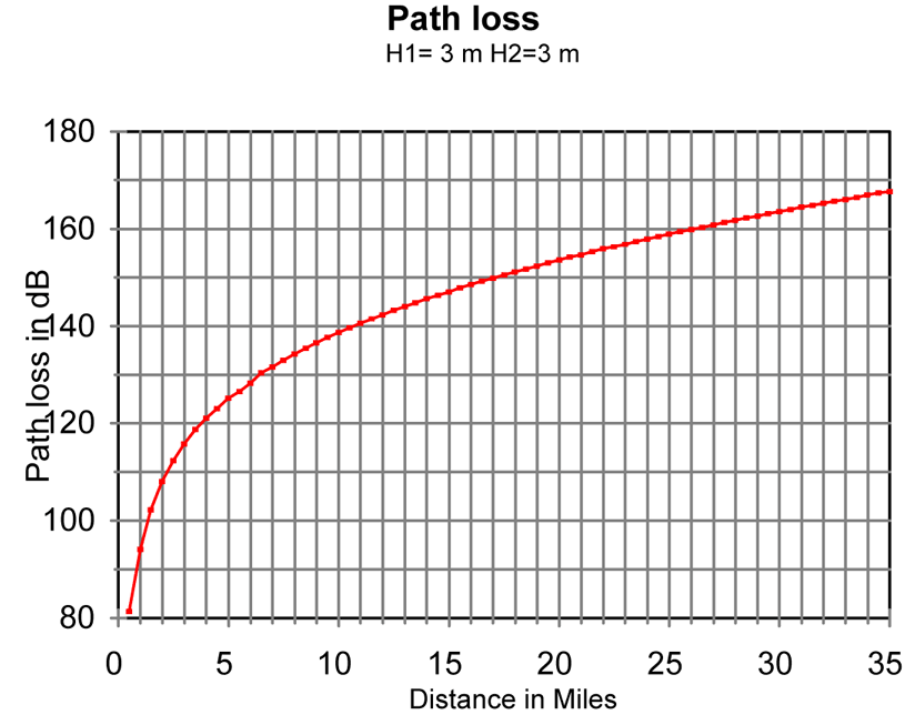
Figure 3. Graph of calculated path loss versus distance for two antennas of 3-meter height, 157-MHz, over seawater. From NTIA TR 97-343.
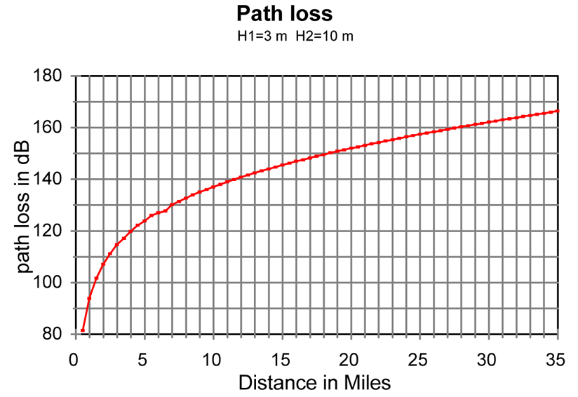
Figure 4. Graph of calculated path loss versus distance for two antennas of 3-meter height and 10-meter height, 157-MHz, over seawater. From NTIA TR 97-343.
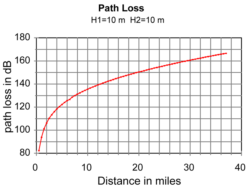
Figure 5. Graph of calculated path loss versus distance for two antennas of 10-meter height, 157-MHz, over seawater. From NTIA TR 97-343.
The case for two recreational vessel, antenna height of 3-meters, is shown in Figure 3. At a distance of 15-miles the calculated path loss is about -148 dB. Assuming 25-Watt transmit power (+44 dBm), -1 dB feedline loss, and 3 dB antenna gain, the transmitter signal is then +46 dBm. With -148 dB path loss, the signal arrives at the other station at a level of -102 dBm. Assuming another 3 dB gain antenna and -1 dB transmission line loss, we have -100 dBm at the receiver input. With a typical receiver sensitivity of 1 μVolt (50-Ohm antenna) or -107 dBm, the received signal should be at least 7 dB above the receiver minimum sensitivity for good signal-to-noise on the recovered modulation. Communication should be possible 50-percent of the time, the metric of the calculation method. Note that the method assumes a smooth earth model with no intervening terrain and conductivity of seawater.
Comparing the above with a calculation for two antennas at 10-meters, at the same 15-miles the path loss is -144 dB. This is an improvement of 4 dB. We see that increasing antenna height by a factor of about three decreases path loss by 4 dB. While signal strenth has improved with added height, it is not as significant as in other models. Tripling height increased signal by 2.5-times (4 dB).
This model is also quite different in its prediction of path loss increase with distance increase. Once the path distance is more than about 10-miles, the model predicts that the path loss will increase by 1-dB for each additional mile, at least out to the limit of the graphed distance, about 35-miles
As I noted above, three models show antenna height has a generous effect on signal strength: every time antenna height is doubled, received signal strength increases four times (or 6 dB). The NTIA model was less generous with height; 3-times increase in antenna height only improved the signal 2.5-times (4 dB).
The influence of antenna height seems very significant in three of the four methods of predicting radio propagation and still effective in the fourth method. This seems to suggest that antenna height really is very important, particularly when it is possible without too much mechanical difficulty to create a doubling of the antenna height, as would occur, say, if an antenna were raised to 10-feet from 5-feet in height. There is evidence in both the FCC data, Egli's data, and the ITU data that such an antenna height increase will pay back a substantial dividend in increased signal and thus increased range.
On this basis, it seems that one ought to prefer height to antenna gain in most instances. For example, it would be better to raise an antenna of 3-dB gain to double the height of an antenna of 6-dB gain. The increase in height is predicted to return a 6-dB increase in gain over most signal paths, while the increase in antenna gain would only return 3-dB (and then only in the main lobe which must be pointed at the distance station to achieve the gain).
All four models also point to the effect of distance on path loss as being much greater than the theoretical free space model. In the free space model signal strength decreases with the square of the distance, that is, if the distance is doubled the signal decreases by a factor of 1/4 in strength. The models show that actual real world radio propagation causes signal strength to decrease at a much faster rate. If the distance is doubled, the signal strength decreases by a factor of 1/16 for shorter distances; over longer distances the rate of signal strength decrease is even faster with increasing distance, on the order of a decrease by 1/32 for a doubling of distance.
The four models examined in this review are all respected models. The FCC model is used to establish the authorized power for stations in the Maritime Service. Egli's model is taught in university courses on radio propagation (although perhaps today more modern methods have supplanted it). And the ITU recommendation is used to establish transmitter power necessary for many important radio services, including the AIS System. These models are better tools for estimating radio range than the simple method of predicting the radio horizon distance based on antenna elevation to establish a so-called line-of-sight path. The NTIA model is used in their technical reports.
If this article has raised any questions or if you have a comment, feel free to post it to a discussion thread reserved for that purpose.
Copyright © 2017 by James W. Hebert. Unauthorized reproduction prohibited.
This is a verified HTML 4.01 document served to you from continuousWave
Author: James W. Hebert
This article first appeared March 12, 2017. An earlier version appeared in a thread of articles in 2013
